Finetuning Torchvision Models

Author: Nathan Inkawhich

In this tutorial we will take a deeper look at how to finetune and feature extract the torchvision models, all of which have been pretrained on the 1000-class Imagenet dataset. This tutorial will give an indepth look at how to work with several modern CNN architectures, and will build an intuition for finetuning any PyTorch model. Since each model architecture is different, there is no boilerplate finetuning code that will work in all scenarios. Rather, the researcher must look at the existing architecture and make custom adjustments for each model.

In this document we will perform two types of transfer learning: finetuning and feature extraction. In finetuning, we start with a pretrained model and update all of the model’s parameters for our new task, in essence retraining the whole model. In feature extraction, we start with a pretrained model and only update the final layer weights from which we derive predictions. It is called feature extraction because we use the pretrained CNN as a fixed feature-extractor, and only change the output layer. For more technical information about transfer learning see here and here.

In general both transfer learning methods follow the same few steps:

• Initialize the pretrained model
• Reshape the final layer(s) to have the same number of outputs as the number of classes in the new dataset
• Define for the optimization algorithm which parameters we want to update during training
• Run the training step

from __future__ import print_function
from __future__ import division
import torch
import torch.nn as nn
import torch.optim as optim
import numpy as np
import torchvision
from torchvision import datasets, models, transforms
import matplotlib.pyplot as plt
import time
import os
import copy
print("PyTorch Version: ",torch.__version__)
print("Torchvision Version: ",torchvision.__version__)

Out:

PyTorch Version:  1.0.0.dev20181128
Torchvision Version:  0.2.1

Inputs

Here are all of the parameters to change for the run. We will use the hymenoptera_data dataset which can be downloaded here. This dataset contains two classes, bees and ants, and is structured such that we can use the ImageFolder dataset, rather than writing our own custom dataset. Download the data and set the data_dir input to the root directory of the dataset. The model_name input is the name of the model you wish to use and must be selected from this list:

[resnet, alexnet, vgg, squeezenet, densenet, inception]

The other inputs are as follows: num_classes is the number of classes in the dataset, batch_size is the batch size used for training and may be adjusted according to the capability of your machine, num_epochs is the number of training epochs we want to run, and feature_extract is a boolean that defines if we are finetuning or feature extracting. If feature_extract = False, the model is finetuned and all model parameters are updated. If feature_extract = True, only the last layer parameters are updated, the others remain fixed.

# Top level data directory. Here we assume the format of the directory conforms
#   to the ImageFolder structure
data_dir = "./hymenoptera_data"

# Models to choose from [resnet, alexnet, vgg, squeezenet, densenet, inception]
model_name = "squeezenet"

# Number of classes in the dataset
num_classes = 2

# Batch size for training (change depending on how much memory you have)
batch_size = 8

# Number of epochs to train for
num_epochs = 15

# Flag for feature extracting. When False, we finetune the whole model,
#   when True we only update the reshaped layer params
feature_extract = True

Helper Functions

Before we write the code for adjusting the models, lets define a few helper functions.

Model Training and Validation Code

The train_model function handles the training and validation of a given model. As input, it takes a PyTorch model, a dictionary of dataloaders, a loss function, an optimizer, a specified number of epochs to train and validate for, and a boolean flag for when the model is an Inception model. The is_inception flag is used to accomodate the Inception v3 model, as that architecture uses an auxiliary output and the overall model loss respects both the auxiliary output and the final output, as described here. The function trains for the specified number of epochs and after each epoch runs a full validation step. It also keeps track of the best performing model (in terms of validation accuracy), and at the end of training returns the best performing model. After each epoch, the training and validation accuracies are printed.

def train_model(model, dataloaders, criterion, optimizer, num_epochs=25, is_inception=False):
    since = time.time()

    val_acc_history = []

    best_model_wts = copy.deepcopy(model.state_dict())
    best_acc = 0.0

    for epoch in range(num_epochs):
        print('Epoch {}/{}'.format(epoch, num_epochs - 1))
        print('-' * 10)

        # Each epoch has a training and validation phase
        for phase in ['train', 'val']:
            if phase == 'train':
                model.train()  # Set model to training mode
            else:
                model.eval()   # Set model to evaluate mode

            running_loss = 0.0
            running_corrects = 0

            # Iterate over data.
            for inputs, labels in dataloaders[phase]:
                inputs = inputs.to(device)
                labels = labels.to(device)

                # zero the parameter gradients
                optimizer.zero_grad()

                # forward
                # track history if only in train
                with torch.set_grad_enabled(phase == 'train'):
                    # Get model outputs and calculate loss
                    # Special case for inception because in training it has an auxiliary output. In train
                    #   mode we calculate the loss by summing the final output and the auxiliary output
                    #   but in testing we only consider the final output.
                    if is_inception and phase == 'train':
                        # From https://discuss.pytorch.org/t/how-to-optimize-inception-model-with-auxiliary-classifiers/7958
                        outputs, aux_outputs = model(inputs)
                        loss1 = criterion(outputs, labels)
                        loss2 = criterion(aux_outputs, labels)
                        loss = loss1 + 0.4*loss2
                    else:
                        outputs = model(inputs)
                        loss = criterion(outputs, labels)

                    _, preds = torch.max(outputs, 1)

                    # backward + optimize only if in training phase
                    if phase == 'train':
                        loss.backward()
                        optimizer.step()

                # statistics
                running_loss += loss.item() * inputs.size(0)
                running_corrects += torch.sum(preds == labels.data)

            epoch_loss = running_loss / len(dataloaders[phase].dataset)
            epoch_acc = running_corrects.double() / len(dataloaders[phase].dataset)

            print('{} Loss: {:.4f} Acc: {:.4f}'.format(phase, epoch_loss, epoch_acc))

            # deep copy the model
            if phase == 'val' and epoch_acc > best_acc:
                best_acc = epoch_acc
                best_model_wts = copy.deepcopy(model.state_dict())
            if phase == 'val':
                val_acc_history.append(epoch_acc)

        print()

    time_elapsed = time.time() - since
    print('Training complete in {:.0f}m {:.0f}s'.format(time_elapsed // 60, time_elapsed % 60))
    print('Best val Acc: {:4f}'.format(best_acc))

    # load best model weights
    model.load_state_dict(best_model_wts)
    return model, val_acc_history

Set Model Parameters’ .requires_grad attribute

This helper function sets the .requires_grad attribute of the parameters in the model to False when we are feature extracting. By default, when we load a pretrained model all of the parameters have .requires_grad=True, which is fine if we are training from scratch or finetuning. However, if we are feature extracting and only want to compute gradients for the newly initialized layer then we want all of the other parameters to not require gradients. This will make more sense later.

def set_parameter_requires_grad(model, feature_extracting):
    if feature_extracting:
        for param in model.parameters():
            param.requires_grad = False

Initialize and Reshape the Networks

Now to the most interesting part. Here is where we handle the reshaping of each network. Note, this is not an automatic procedure and is unique to each model. Recall, the final layer of a CNN model, which is often times an FC layer, has the same number of nodes as the number of output classes in the dataset. Since all of the models have been pretrained on Imagenet, they all have output layers of size 1000, one node for each class. The goal here is to reshape the last layer to have the same number of inputs as before, AND to have the same number of outputs as the number of classes in the dataset. In the following sections we will discuss how to alter the architecture of each model individually. But first, there is one important detail regarding the difference between finetuning and feature-extraction.

When feature extracting, we only want to update the parameters of the last layer, or in other words, we only want to update the parameters for the layer(s) we are reshaping. Therefore, we do not need to compute the gradients of the parameters that we are not changing, so for efficiency we set the .requires_grad attribute to False. This is important because by default, this attribute is set to True. Then, when we initialize the new layer and by default the new parameters have .requires_grad=True so only the new layer’s parameters will be updated. When we are finetuning we can leave all of the .required_grad’s set to the default of True.

Finally, notice that inception_v3 requires the input size to be (299,299), whereas all of the other models expect (224,224).

Resnet

Resnet was introduced in the paper Deep Residual Learning for Image Recognition. There are several variants of different sizes, including Resnet18, Resnet34, Resnet50, Resnet101, and Resnet152, all of which are available from torchvision models. Here we use Resnet18, as our dataset is small and only has two classes. When we print the model, we see that the last layer is a fully connected layer as shown below:

(fc): Linear(in_features=512, out_features=1000, bias=True)

Thus, we must reinitialize model.fc to be a Linear layer with 512 input features and 2 output features with:

model.fc = nn.Linear(512, num_classes)

Alexnet

Alexnet was introduced in the paper ImageNet Classification with Deep Convolutional Neural Networks and was the first very successful CNN on the ImageNet dataset. When we print the model architecture, we see the model output comes from the 6th layer of the classifier

(classifier): Sequential(
    ...
    (6): Linear(in_features=4096, out_features=1000, bias=True)
 )

To use the model with our dataset we reinitialize this layer as

model.classifier[6] = nn.Linear(4096,num_classes)

VGG

VGG was introduced in the paper Very Deep Convolutional Networks for Large-Scale Image Recognition. Torchvision offers eight versions of VGG with various lengths and some that have batch normalizations layers. Here we use VGG-11 with batch normalization. The output layer is similar to Alexnet, i.e.

(classifier): Sequential(
    ...
    (6): Linear(in_features=4096, out_features=1000, bias=True)
 )

Therefore, we use the same technique to modify the output layer

model.classifier[6] = nn.Linear(4096,num_classes)

Squeezenet

The Squeeznet architecture is described in the paper SqueezeNet: AlexNet-level accuracy with 50x fewer parameters and <0.5MB model size and uses a different output structure than any of the other models shown here. Torchvision has two versions of Squeezenet, we use version 1.0. The output comes from a 1x1 convolutional layer which is the 1st layer of the classifier:

(classifier): Sequential(
    (0): Dropout(p=0.5)
    (1): Conv2d(512, 1000, kernel_size=(1, 1), stride=(1, 1))
    (2): ReLU(inplace)
    (3): AvgPool2d(kernel_size=13, stride=1, padding=0)
 )

To modify the network, we reinitialize the Conv2d layer to have an output feature map of depth 2 as

model.classifier[1] = nn.Conv2d(512, num_classes, kernel_size=(1,1), stride=(1,1))

Densenet

Densenet was introduced in the paper Densely Connected Convolutional Networks. Torchvision has four variants of Densenet but here we only use Densenet-121. The output layer is a linear layer with 1024 input features:

(classifier): Linear(in_features=1024, out_features=1000, bias=True)

To reshape the network, we reinitialize the classifier’s linear layer as

model.classifier = nn.Linear(1024, num_classes)

Inception v3

Finally, Inception v3 was first described in Rethinking the Inception Architecture for Computer Vision. This network is unique because it has two output layers when training. The second output is known as an auxiliary output and is contained in the AuxLogits part of the network. The primary output is a linear layer at the end of the network. Note, when testing we only consider the primary output. The auxiliary output and primary output of the loaded model are printed as:

(AuxLogits): InceptionAux(
    ...
    (fc): Linear(in_features=768, out_features=1000, bias=True)
 )
 ...
(fc): Linear(in_features=2048, out_features=1000, bias=True)

To finetune this model we must reshape both layers. This is accomplished with the following

model.AuxLogits.fc = nn.Linear(768, num_classes)
model.fc = nn.Linear(2048, num_classes)

Notice, many of the models have similar output structures, but each must be handled slightly differently. Also, check out the printed model architecture of the reshaped network and make sure the number of output features is the same as the number of classes in the dataset.

def initialize_model(model_name, num_classes, feature_extract, use_pretrained=True):
    # Initialize these variables which will be set in this if statement. Each of these
    #   variables is model specific.
    model_ft = None
    input_size = 0

    if model_name == "resnet":
        """ Resnet18
        """
        model_ft = models.resnet18(pretrained=use_pretrained)
        set_parameter_requires_grad(model_ft, feature_extract)
        num_ftrs = model_ft.fc.in_features
        model_ft.fc = nn.Linear(num_ftrs, num_classes)
        input_size = 224

    elif model_name == "alexnet":
        """ Alexnet
        """
        model_ft = models.alexnet(pretrained=use_pretrained)
        set_parameter_requires_grad(model_ft, feature_extract)
        num_ftrs = model_ft.classifier[6].in_features
        model_ft.classifier[6] = nn.Linear(num_ftrs,num_classes)
        input_size = 224

    elif model_name == "vgg":
        """ VGG11_bn
        """
        model_ft = models.vgg11_bn(pretrained=use_pretrained)
        set_parameter_requires_grad(model_ft, feature_extract)
        num_ftrs = model_ft.classifier[6].in_features
        model_ft.classifier[6] = nn.Linear(num_ftrs,num_classes)
        input_size = 224

    elif model_name == "squeezenet":
        """ Squeezenet
        """
        model_ft = models.squeezenet1_0(pretrained=use_pretrained)
        set_parameter_requires_grad(model_ft, feature_extract)
        model_ft.classifier[1] = nn.Conv2d(512, num_classes, kernel_size=(1,1), stride=(1,1))
        model_ft.num_classes = num_classes
        input_size = 224

    elif model_name == "densenet":
        """ Densenet
        """
        model_ft = models.densenet121(pretrained=use_pretrained)
        set_parameter_requires_grad(model_ft, feature_extract)
        num_ftrs = model_ft.classifier.in_features
        model_ft.classifier = nn.Linear(num_ftrs, num_classes)
        input_size = 224

    elif model_name == "inception":
        """ Inception v3
        Be careful, expects (299,299) sized images and has auxiliary output
        """
        model_ft = models.inception_v3(pretrained=use_pretrained)
        set_parameter_requires_grad(model_ft, feature_extract)
        # Handle the auxilary net
        num_ftrs = model_ft.AuxLogits.fc.in_features
        model_ft.AuxLogits.fc = nn.Linear(num_ftrs, num_classes)
        # Handle the primary net
        num_ftrs = model_ft.fc.in_features
        model_ft.fc = nn.Linear(num_ftrs,num_classes)
        input_size = 299

    else:
        print("Invalid model name, exiting...")
        exit()

    return model_ft, input_size

# Initialize the model for this run
model_ft, input_size = initialize_model(model_name, num_classes, feature_extract, use_pretrained=True)

# Print the model we just instantiated
print(model_ft)

Out:

SqueezeNet(
  (features): Sequential(
    (0): Conv2d(3, 96, kernel_size=(7, 7), stride=(2, 2))
    (1): ReLU(inplace)
    (2): MaxPool2d(kernel_size=3, stride=2, padding=0, dilation=1, ceil_mode=True)
    (3): Fire(
      (squeeze): Conv2d(96, 16, kernel_size=(1, 1), stride=(1, 1))
      (squeeze_activation): ReLU(inplace)
      (expand1x1): Conv2d(16, 64, kernel_size=(1, 1), stride=(1, 1))
      (expand1x1_activation): ReLU(inplace)
      (expand3x3): Conv2d(16, 64, kernel_size=(3, 3), stride=(1, 1), padding=(1, 1))
      (expand3x3_activation): ReLU(inplace)
    )
    (4): Fire(
      (squeeze): Conv2d(128, 16, kernel_size=(1, 1), stride=(1, 1))
      (squeeze_activation): ReLU(inplace)
      (expand1x1): Conv2d(16, 64, kernel_size=(1, 1), stride=(1, 1))
      (expand1x1_activation): ReLU(inplace)
      (expand3x3): Conv2d(16, 64, kernel_size=(3, 3), stride=(1, 1), padding=(1, 1))
      (expand3x3_activation): ReLU(inplace)
    )
    (5): Fire(
      (squeeze): Conv2d(128, 32, kernel_size=(1, 1), stride=(1, 1))
      (squeeze_activation): ReLU(inplace)
      (expand1x1): Conv2d(32, 128, kernel_size=(1, 1), stride=(1, 1))
      (expand1x1_activation): ReLU(inplace)
      (expand3x3): Conv2d(32, 128, kernel_size=(3, 3), stride=(1, 1), padding=(1, 1))
      (expand3x3_activation): ReLU(inplace)
    )
    (6): MaxPool2d(kernel_size=3, stride=2, padding=0, dilation=1, ceil_mode=True)
    (7): Fire(
      (squeeze): Conv2d(256, 32, kernel_size=(1, 1), stride=(1, 1))
      (squeeze_activation): ReLU(inplace)
      (expand1x1): Conv2d(32, 128, kernel_size=(1, 1), stride=(1, 1))
      (expand1x1_activation): ReLU(inplace)
      (expand3x3): Conv2d(32, 128, kernel_size=(3, 3), stride=(1, 1), padding=(1, 1))
      (expand3x3_activation): ReLU(inplace)
    )
    (8): Fire(
      (squeeze): Conv2d(256, 48, kernel_size=(1, 1), stride=(1, 1))
      (squeeze_activation): ReLU(inplace)
      (expand1x1): Conv2d(48, 192, kernel_size=(1, 1), stride=(1, 1))
      (expand1x1_activation): ReLU(inplace)
      (expand3x3): Conv2d(48, 192, kernel_size=(3, 3), stride=(1, 1), padding=(1, 1))
      (expand3x3_activation): ReLU(inplace)
    )
    (9): Fire(
      (squeeze): Conv2d(384, 48, kernel_size=(1, 1), stride=(1, 1))
      (squeeze_activation): ReLU(inplace)
      (expand1x1): Conv2d(48, 192, kernel_size=(1, 1), stride=(1, 1))
      (expand1x1_activation): ReLU(inplace)
      (expand3x3): Conv2d(48, 192, kernel_size=(3, 3), stride=(1, 1), padding=(1, 1))
      (expand3x3_activation): ReLU(inplace)
    )
    (10): Fire(
      (squeeze): Conv2d(384, 64, kernel_size=(1, 1), stride=(1, 1))
      (squeeze_activation): ReLU(inplace)
      (expand1x1): Conv2d(64, 256, kernel_size=(1, 1), stride=(1, 1))
      (expand1x1_activation): ReLU(inplace)
      (expand3x3): Conv2d(64, 256, kernel_size=(3, 3), stride=(1, 1), padding=(1, 1))
      (expand3x3_activation): ReLU(inplace)
    )
    (11): MaxPool2d(kernel_size=3, stride=2, padding=0, dilation=1, ceil_mode=True)
    (12): Fire(
      (squeeze): Conv2d(512, 64, kernel_size=(1, 1), stride=(1, 1))
      (squeeze_activation): ReLU(inplace)
      (expand1x1): Conv2d(64, 256, kernel_size=(1, 1), stride=(1, 1))
      (expand1x1_activation): ReLU(inplace)
      (expand3x3): Conv2d(64, 256, kernel_size=(3, 3), stride=(1, 1), padding=(1, 1))
      (expand3x3_activation): ReLU(inplace)
    )
  )
  (classifier): Sequential(
    (0): Dropout(p=0.5)
    (1): Conv2d(512, 2, kernel_size=(1, 1), stride=(1, 1))
    (2): ReLU(inplace)
    (3): AdaptiveAvgPool2d(output_size=(1, 1))
  )
)

Load Data

Now that we know what the input size must be, we can initialize the data transforms, image datasets, and the dataloaders. Notice, the models were pretrained with the hard-coded normalization values, as described here.

# Data augmentation and normalization for training
# Just normalization for validation
data_transforms = {
    'train': transforms.Compose([
        transforms.RandomResizedCrop(input_size),
        transforms.RandomHorizontalFlip(),
        transforms.ToTensor(),
        transforms.Normalize([0.485, 0.456, 0.406], [0.229, 0.224, 0.225])
    ]),
    'val': transforms.Compose([
        transforms.Resize(input_size),
        transforms.CenterCrop(input_size),
        transforms.ToTensor(),
        transforms.Normalize([0.485, 0.456, 0.406], [0.229, 0.224, 0.225])
    ]),
}

print("Initializing Datasets and Dataloaders...")

# Create training and validation datasets
image_datasets = {x: datasets.ImageFolder(os.path.join(data_dir, x), data_transforms[x]) for x in ['train', 'val']}
# Create training and validation dataloaders
dataloaders_dict = {x: torch.utils.data.DataLoader(image_datasets[x], batch_size=batch_size, shuffle=True, num_workers=4) for x in ['train', 'val']}

# Detect if we have a GPU available
device = torch.device("cuda:0" if torch.cuda.is_available() else "cpu")

Out:

Initializing Datasets and Dataloaders...

Create the Optimizer

Now that the model structure is correct, the final step for finetuning and feature extracting is to create an optimizer that only updates the desired parameters. Recall that after loading the pretrained model, but before reshaping, if feature_extract=True we manually set all of the parameter’s .requires_grad attributes to False. Then the reinitialized layer’s parameters have .requires_grad=True by default. So now we know that all parameters that have .requires_grad=True should be optimized. Next, we make a list of such parameters and input this list to the SGD algorithm constructor.

To verify this, check out the printed parameters to learn. When finetuning, this list should be long and include all of the model parameters. However, when feature extracting this list should be short and only include the weights and biases of the reshaped layers.

# Send the model to GPU
model_ft = model_ft.to(device)

# Gather the parameters to be optimized/updated in this run. If we are
#  finetuning we will be updating all parameters. However, if we are
#  doing feature extract method, we will only update the parameters
#  that we have just initialized, i.e. the parameters with requires_grad
#  is True.
params_to_update = model_ft.parameters()
print("Params to learn:")
if feature_extract:
    params_to_update = []
    for name,param in model_ft.named_parameters():
        if param.requires_grad == True:
            params_to_update.append(param)
            print("\t",name)
else:
    for name,param in model_ft.named_parameters():
        if param.requires_grad == True:
            print("\t",name)

# Observe that all parameters are being optimized
optimizer_ft = optim.SGD(params_to_update, lr=0.001, momentum=0.9)

Out:

Params to learn:
         classifier.1.weight
         classifier.1.bias

Run Training and Validation Step

Finally, the last step is to setup the loss for the model, then run the training and validation function for the set number of epochs. Notice, depending on the number of epochs this step may take a while on a CPU. Also, the default learning rate is not optimal for all of the models, so to achieve maximum accuracy it would be necessary to tune for each model separately.

# Setup the loss fxn
criterion = nn.CrossEntropyLoss()

# Train and evaluate
model_ft, hist = train_model(model_ft, dataloaders_dict, criterion, optimizer_ft, num_epochs=num_epochs, is_inception=(model_name=="inception"))

Out:

Epoch 0/14
----------
train Loss: 0.5176 Acc: 0.7664
val Loss: 0.3147 Acc: 0.9020

Epoch 1/14
----------
train Loss: 0.2813 Acc: 0.8975
val Loss: 0.2945 Acc: 0.9150

Epoch 2/14
----------
train Loss: 0.2146 Acc: 0.9057
val Loss: 0.2933 Acc: 0.9085

Epoch 3/14
----------
train Loss: 0.1909 Acc: 0.9262
val Loss: 0.2711 Acc: 0.9281

Epoch 4/14
----------
train Loss: 0.1911 Acc: 0.9139
val Loss: 0.2665 Acc: 0.9281

Epoch 5/14
----------
train Loss: 0.1514 Acc: 0.9262
val Loss: 0.2724 Acc: 0.9216

Epoch 6/14
----------
train Loss: 0.1847 Acc: 0.9303
val Loss: 0.2922 Acc: 0.9216

Epoch 7/14
----------
train Loss: 0.1551 Acc: 0.9344
val Loss: 0.2915 Acc: 0.9150

Epoch 8/14
----------
train Loss: 0.1463 Acc: 0.9303
val Loss: 0.3278 Acc: 0.9150

Epoch 9/14
----------
train Loss: 0.1574 Acc: 0.9426
val Loss: 0.2975 Acc: 0.9216

Epoch 10/14
----------
train Loss: 0.1775 Acc: 0.9303
val Loss: 0.2908 Acc: 0.9281

Epoch 11/14
----------
train Loss: 0.1150 Acc: 0.9672
val Loss: 0.2971 Acc: 0.9346

Epoch 12/14
----------
train Loss: 0.1018 Acc: 0.9508
val Loss: 0.3148 Acc: 0.9216

Epoch 13/14
----------
train Loss: 0.1648 Acc: 0.9057
val Loss: 0.3816 Acc: 0.8954

Epoch 14/14
----------
train Loss: 0.1610 Acc: 0.9467
val Loss: 0.3417 Acc: 0.9216

Training complete in 0m 22s
Best val Acc: 0.934641

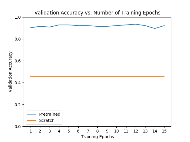
Comparison with Model Trained from Scratch

Just for fun, lets see how the model learns if we do not use transfer learning. The performance of finetuning vs. feature extracting depends largely on the dataset but in general both transfer learning methods produce favorable results in terms of training time and overall accuracy versus a model trained from scratch.

# Initialize the non-pretrained version of the model used for this run
scratch_model,_ = initialize_model(model_name, num_classes, feature_extract=False, use_pretrained=False)
scratch_model = scratch_model.to(device)
scratch_optimizer = optim.SGD(scratch_model.parameters(), lr=0.001, momentum=0.9)
scratch_criterion = nn.CrossEntropyLoss()
_,scratch_hist = train_model(scratch_model, dataloaders_dict, scratch_criterion, scratch_optimizer, num_epochs=num_epochs, is_inception=(model_name=="inception"))

# Plot the training curves of validation accuracy vs. number
#  of training epochs for the transfer learning method and
#  the model trained from scratch
ohist = []
shist = []

ohist = [h.cpu().numpy() for h in hist]
shist = [h.cpu().numpy() for h in scratch_hist]

plt.title("Validation Accuracy vs. Number of Training Epochs")
plt.xlabel("Training Epochs")
plt.ylabel("Validation Accuracy")
plt.plot(range(1,num_epochs+1),ohist,label="Pretrained")
plt.plot(range(1,num_epochs+1),shist,label="Scratch")
plt.ylim((0,1.))
plt.xticks(np.arange(1, num_epochs+1, 1.0))
plt.legend()
plt.show()

Out:

Epoch 0/14
----------
train Loss: 0.6997 Acc: 0.4672
val Loss: 0.6931 Acc: 0.4575

Epoch 1/14
----------
train Loss: 0.6899 Acc: 0.5041
val Loss: 0.6939 Acc: 0.4575

Epoch 2/14
----------
train Loss: 0.6849 Acc: 0.5041
val Loss: 0.6931 Acc: 0.4575

Epoch 3/14
----------
train Loss: 0.6931 Acc: 0.5000
val Loss: 0.6931 Acc: 0.4575

Epoch 4/14
----------
train Loss: 0.6922 Acc: 0.5000
val Loss: 0.6931 Acc: 0.4575

Epoch 5/14
----------
train Loss: 0.6845 Acc: 0.5041
val Loss: 0.7029 Acc: 0.4575

Epoch 6/14
----------
train Loss: 0.6940 Acc: 0.5082
val Loss: 0.6931 Acc: 0.4575

Epoch 7/14
----------
train Loss: 0.6931 Acc: 0.5041
val Loss: 0.6931 Acc: 0.4575

Epoch 8/14
----------
train Loss: 0.6931 Acc: 0.5041
val Loss: 0.6931 Acc: 0.4575

Epoch 9/14
----------
train Loss: 0.6932 Acc: 0.4959
val Loss: 0.6931 Acc: 0.4575

Epoch 10/14
----------
train Loss: 0.6931 Acc: 0.5041
val Loss: 0.6931 Acc: 0.4575

Epoch 11/14
----------
train Loss: 0.6932 Acc: 0.5000
val Loss: 0.6931 Acc: 0.4575

Epoch 12/14
----------
train Loss: 0.6932 Acc: 0.5000
val Loss: 0.6931 Acc: 0.4575

Epoch 13/14
----------
train Loss: 0.6931 Acc: 0.5041
val Loss: 0.6931 Acc: 0.4575

Epoch 14/14
----------
train Loss: 0.6931 Acc: 0.5123
val Loss: 0.6931 Acc: 0.4575

Training complete in 0m 32s
Best val Acc: 0.457516

Final Thoughts and Where to Go Next

Try running some of the other models and see how good the accuracy gets. Also, notice that feature extracting takes less time because in the backward pass we do not have to calculate most of the gradients. There are many places to go from here. You could:

• Run this code with a harder dataset and see some more benefits of transfer learning
• Using the methods described here, use transfer learning to update a different model, perhaps in a new domain (i.e. NLP, audio, etc.)
• Once you are happy with a model, you can export it as an ONNX model, or trace it using the hybrid frontend for more speed and optimization opportunities.

Total running time of the script: ( 0 minutes 54.503 seconds)