Spatial Transformer Networks Tutorial

Author: Ghassen HAMROUNI

In this tutorial, you will learn how to augment your network using a visual attention mechanism called spatial transformer networks. You can read more about the spatial transformer networks in the DeepMind paper

Spatial transformer networks are a generalization of differentiable attention to any spatial transformation. Spatial transformer networks (STN for short) allow a neural network to learn how to perform spatial transformations on the input image in order to enhance the geometric invariance of the model. For example, it can crop a region of interest, scale and correct the orientation of an image. It can be a useful mechanism because CNNs are not invariant to rotation and scale and more general affine transformations.

One of the best things about STN is the ability to simply plug it into any existing CNN with very little modification.

# License: BSD
# Author: Ghassen Hamrouni

from __future__ import print_function
import torch
import torch.nn as nn
import torch.nn.functional as F
import torch.optim as optim
import torchvision
from torchvision import datasets, transforms
import matplotlib.pyplot as plt
import numpy as np

plt.ion()   # interactive mode

Loading the data

In this post we experiment with the classic MNIST dataset. Using a standard convolutional network augmented with a spatial transformer network.

device = torch.device("cuda" if torch.cuda.is_available() else "cpu")

# Training dataset
train_loader = torch.utils.data.DataLoader(
    datasets.MNIST(root='.', train=True, download=True,
                   transform=transforms.Compose([
                       transforms.ToTensor(),
                       transforms.Normalize((0.1307,), (0.3081,))
                   ])), batch_size=64, shuffle=True, num_workers=4)
# Test dataset
test_loader = torch.utils.data.DataLoader(
    datasets.MNIST(root='.', train=False, transform=transforms.Compose([
        transforms.ToTensor(),
        transforms.Normalize((0.1307,), (0.3081,))
    ])), batch_size=64, shuffle=True, num_workers=4)

Out:

Downloading http://yann.lecun.com/exdb/mnist/train-images-idx3-ubyte.gz to ./MNIST/raw/train-images-idx3-ubyte.gz
Extracting ./MNIST/raw/train-images-idx3-ubyte.gz
Downloading http://yann.lecun.com/exdb/mnist/train-labels-idx1-ubyte.gz to ./MNIST/raw/train-labels-idx1-ubyte.gz
Extracting ./MNIST/raw/train-labels-idx1-ubyte.gz
Downloading http://yann.lecun.com/exdb/mnist/t10k-images-idx3-ubyte.gz to ./MNIST/raw/t10k-images-idx3-ubyte.gz
Extracting ./MNIST/raw/t10k-images-idx3-ubyte.gz
Downloading http://yann.lecun.com/exdb/mnist/t10k-labels-idx1-ubyte.gz to ./MNIST/raw/t10k-labels-idx1-ubyte.gz
Extracting ./MNIST/raw/t10k-labels-idx1-ubyte.gz
Processing...
Done!

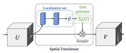
Depicting spatial transformer networks

Spatial transformer networks boils down to three main components :

• The localization network is a regular CNN which regresses the transformation parameters. The transformation is never learned explicitly from this dataset, instead the network learns automatically the spatial transformations that enhances the global accuracy.
• The grid generator generates a grid of coordinates in the input image corresponding to each pixel from the output image.
• The sampler uses the parameters of the transformation and applies it to the input image.

Note

We need the latest version of PyTorch that contains affine_grid and grid_sample modules.

class Net(nn.Module):
    def __init__(self):
        super(Net, self).__init__()
        self.conv1 = nn.Conv2d(1, 10, kernel_size=5)
        self.conv2 = nn.Conv2d(10, 20, kernel_size=5)
        self.conv2_drop = nn.Dropout2d()
        self.fc1 = nn.Linear(320, 50)
        self.fc2 = nn.Linear(50, 10)

        # Spatial transformer localization-network
        self.localization = nn.Sequential(
            nn.Conv2d(1, 8, kernel_size=7),
            nn.MaxPool2d(2, stride=2),
            nn.ReLU(True),
            nn.Conv2d(8, 10, kernel_size=5),
            nn.MaxPool2d(2, stride=2),
            nn.ReLU(True)
        )

        # Regressor for the 3 * 2 affine matrix
        self.fc_loc = nn.Sequential(
            nn.Linear(10 * 3 * 3, 32),
            nn.ReLU(True),
            nn.Linear(32, 3 * 2)
        )

        # Initialize the weights/bias with identity transformation
        self.fc_loc[2].weight.data.zero_()
        self.fc_loc[2].bias.data.copy_(torch.tensor([1, 0, 0, 0, 1, 0], dtype=torch.float))

    # Spatial transformer network forward function
    def stn(self, x):
        xs = self.localization(x)
        xs = xs.view(-1, 10 * 3 * 3)
        theta = self.fc_loc(xs)
        theta = theta.view(-1, 2, 3)

        grid = F.affine_grid(theta, x.size())
        x = F.grid_sample(x, grid)

        return x

    def forward(self, x):
        # transform the input
        x = self.stn(x)

        # Perform the usual forward pass
        x = F.relu(F.max_pool2d(self.conv1(x), 2))
        x = F.relu(F.max_pool2d(self.conv2_drop(self.conv2(x)), 2))
        x = x.view(-1, 320)
        x = F.relu(self.fc1(x))
        x = F.dropout(x, training=self.training)
        x = self.fc2(x)
        return F.log_softmax(x, dim=1)


model = Net().to(device)

Training the model

Now, let’s use the SGD algorithm to train the model. The network is learning the classification task in a supervised way. In the same time the model is learning STN automatically in an end-to-end fashion.

optimizer = optim.SGD(model.parameters(), lr=0.01)


def train(epoch):
    model.train()
    for batch_idx, (data, target) in enumerate(train_loader):
        data, target = data.to(device), target.to(device)

        optimizer.zero_grad()
        output = model(data)
        loss = F.nll_loss(output, target)
        loss.backward()
        optimizer.step()
        if batch_idx % 500 == 0:
            print('Train Epoch: {} [{}/{} ({:.0f}%)]\tLoss: {:.6f}'.format(
                epoch, batch_idx * len(data), len(train_loader.dataset),
                100. * batch_idx / len(train_loader), loss.item()))
#
# A simple test procedure to measure STN the performances on MNIST.
#


def test():
    with torch.no_grad():
        model.eval()
        test_loss = 0
        correct = 0
        for data, target in test_loader:
            data, target = data.to(device), target.to(device)
            output = model(data)

            # sum up batch loss
            test_loss += F.nll_loss(output, target, size_average=False).item()
            # get the index of the max log-probability
            pred = output.max(1, keepdim=True)[1]
            correct += pred.eq(target.view_as(pred)).sum().item()

        test_loss /= len(test_loader.dataset)
        print('\nTest set: Average loss: {:.4f}, Accuracy: {}/{} ({:.0f}%)\n'
              .format(test_loss, correct, len(test_loader.dataset),
                      100. * correct / len(test_loader.dataset)))

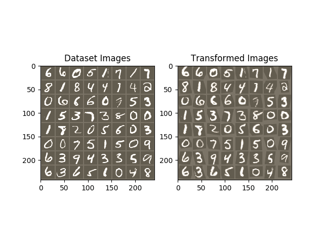
Visualizing the STN results

Now, we will inspect the results of our learned visual attention mechanism.

We define a small helper function in order to visualize the transformations while training.

def convert_image_np(inp):
    """Convert a Tensor to numpy image."""
    inp = inp.numpy().transpose((1, 2, 0))
    mean = np.array([0.485, 0.456, 0.406])
    std = np.array([0.229, 0.224, 0.225])
    inp = std * inp + mean
    inp = np.clip(inp, 0, 1)
    return inp

# We want to visualize the output of the spatial transformers layer
# after the training, we visualize a batch of input images and
# the corresponding transformed batch using STN.


def visualize_stn():
    with torch.no_grad():
        # Get a batch of training data
        data = next(iter(test_loader))[0].to(device)

        input_tensor = data.cpu()
        transformed_input_tensor = model.stn(data).cpu()

        in_grid = convert_image_np(
            torchvision.utils.make_grid(input_tensor))

        out_grid = convert_image_np(
            torchvision.utils.make_grid(transformed_input_tensor))

        # Plot the results side-by-side
        f, axarr = plt.subplots(1, 2)
        axarr[0].imshow(in_grid)
        axarr[0].set_title('Dataset Images')

        axarr[1].imshow(out_grid)
        axarr[1].set_title('Transformed Images')

for epoch in range(1, 20 + 1):
    train(epoch)
    test()

# Visualize the STN transformation on some input batch
visualize_stn()

plt.ioff()
plt.show()

Out:

Train Epoch: 1 [0/60000 (0%)]   Loss: 2.345713
Train Epoch: 1 [32000/60000 (53%)]      Loss: 0.800387

Test set: Average loss: 0.2062, Accuracy: 9431/10000 (94%)

Train Epoch: 2 [0/60000 (0%)]   Loss: 0.353793
Train Epoch: 2 [32000/60000 (53%)]      Loss: 0.311179

Test set: Average loss: 0.1226, Accuracy: 9648/10000 (96%)

Train Epoch: 3 [0/60000 (0%)]   Loss: 0.187958
Train Epoch: 3 [32000/60000 (53%)]      Loss: 0.465108

Test set: Average loss: 0.1741, Accuracy: 9489/10000 (95%)

Train Epoch: 4 [0/60000 (0%)]   Loss: 0.414825
Train Epoch: 4 [32000/60000 (53%)]      Loss: 0.190623

Test set: Average loss: 0.0719, Accuracy: 9775/10000 (98%)

Train Epoch: 5 [0/60000 (0%)]   Loss: 0.326834
Train Epoch: 5 [32000/60000 (53%)]      Loss: 0.207580

Test set: Average loss: 0.0712, Accuracy: 9773/10000 (98%)

Train Epoch: 6 [0/60000 (0%)]   Loss: 0.213898
Train Epoch: 6 [32000/60000 (53%)]      Loss: 0.246923

Test set: Average loss: 0.0848, Accuracy: 9747/10000 (97%)

Train Epoch: 7 [0/60000 (0%)]   Loss: 0.081923
Train Epoch: 7 [32000/60000 (53%)]      Loss: 0.152231

Test set: Average loss: 0.0660, Accuracy: 9808/10000 (98%)

Train Epoch: 8 [0/60000 (0%)]   Loss: 0.131550
Train Epoch: 8 [32000/60000 (53%)]      Loss: 0.176575

Test set: Average loss: 0.0542, Accuracy: 9838/10000 (98%)

Train Epoch: 9 [0/60000 (0%)]   Loss: 0.237464
Train Epoch: 9 [32000/60000 (53%)]      Loss: 0.034639

Test set: Average loss: 0.0516, Accuracy: 9846/10000 (98%)

Train Epoch: 10 [0/60000 (0%)]  Loss: 0.056443
Train Epoch: 10 [32000/60000 (53%)]     Loss: 0.136011

Test set: Average loss: 0.0478, Accuracy: 9842/10000 (98%)

Train Epoch: 11 [0/60000 (0%)]  Loss: 0.197817
Train Epoch: 11 [32000/60000 (53%)]     Loss: 0.065170

Test set: Average loss: 0.0475, Accuracy: 9864/10000 (99%)

Train Epoch: 12 [0/60000 (0%)]  Loss: 0.123880
Train Epoch: 12 [32000/60000 (53%)]     Loss: 0.062649

Test set: Average loss: 0.0628, Accuracy: 9802/10000 (98%)

Train Epoch: 13 [0/60000 (0%)]  Loss: 0.134825
Train Epoch: 13 [32000/60000 (53%)]     Loss: 0.110926

Test set: Average loss: 0.0602, Accuracy: 9810/10000 (98%)

Train Epoch: 14 [0/60000 (0%)]  Loss: 0.069058
Train Epoch: 14 [32000/60000 (53%)]     Loss: 0.094049

Test set: Average loss: 0.0472, Accuracy: 9856/10000 (99%)

Train Epoch: 15 [0/60000 (0%)]  Loss: 0.035787
Train Epoch: 15 [32000/60000 (53%)]     Loss: 0.113708

Test set: Average loss: 0.0480, Accuracy: 9860/10000 (99%)

Train Epoch: 16 [0/60000 (0%)]  Loss: 0.112437
Train Epoch: 16 [32000/60000 (53%)]     Loss: 0.118043

Test set: Average loss: 0.0386, Accuracy: 9885/10000 (99%)

Train Epoch: 17 [0/60000 (0%)]  Loss: 0.090034
Train Epoch: 17 [32000/60000 (53%)]     Loss: 0.300923

Test set: Average loss: 0.0539, Accuracy: 9834/10000 (98%)

Train Epoch: 18 [0/60000 (0%)]  Loss: 0.428552
Train Epoch: 18 [32000/60000 (53%)]     Loss: 0.071741

Test set: Average loss: 0.0536, Accuracy: 9829/10000 (98%)

Train Epoch: 19 [0/60000 (0%)]  Loss: 0.134506
Train Epoch: 19 [32000/60000 (53%)]     Loss: 0.049006

Test set: Average loss: 0.0386, Accuracy: 9876/10000 (99%)

Train Epoch: 20 [0/60000 (0%)]  Loss: 0.091285
Train Epoch: 20 [32000/60000 (53%)]     Loss: 0.068183

Test set: Average loss: 0.0394, Accuracy: 9875/10000 (99%)

Total running time of the script: ( 1 minutes 42.444 seconds)