Transfer Learning Tutorial

Author: Sasank Chilamkurthy

In this tutorial, you will learn how to train your network using transfer learning. You can read more about the transfer learning at cs231n notes

Quoting these notes,

In practice, very few people train an entire Convolutional Network from scratch (with random initialization), because it is relatively rare to have a dataset of sufficient size. Instead, it is common to pretrain a ConvNet on a very large dataset (e.g. ImageNet, which contains 1.2 million images with 1000 categories), and then use the ConvNet either as an initialization or a fixed feature extractor for the task of interest.

These two major transfer learning scenarios look as follows:

• Finetuning the convnet: Instead of random initializaion, we initialize the network with a pretrained network, like the one that is trained on imagenet 1000 dataset. Rest of the training looks as usual.
• ConvNet as fixed feature extractor: Here, we will freeze the weights for all of the network except that of the final fully connected layer. This last fully connected layer is replaced with a new one with random weights and only this layer is trained.

# License: BSD
# Author: Sasank Chilamkurthy

from __future__ import print_function, division

import torch
import torch.nn as nn
import torch.optim as optim
from torch.optim import lr_scheduler
import numpy as np
import torchvision
from torchvision import datasets, models, transforms
import matplotlib.pyplot as plt
import time
import os
import copy

plt.ion()   # interactive mode

Load Data

We will use torchvision and torch.utils.data packages for loading the data.

The problem we’re going to solve today is to train a model to classify ants and bees. We have about 120 training images each for ants and bees. There are 75 validation images for each class. Usually, this is a very small dataset to generalize upon, if trained from scratch. Since we are using transfer learning, we should be able to generalize reasonably well.

This dataset is a very small subset of imagenet.

Note

Download the data from here and extract it to the current directory.

# Data augmentation and normalization for training
# Just normalization for validation
data_transforms = {
    'train': transforms.Compose([
        transforms.RandomResizedCrop(224),
        transforms.RandomHorizontalFlip(),
        transforms.ToTensor(),
        transforms.Normalize([0.485, 0.456, 0.406], [0.229, 0.224, 0.225])
    ]),
    'val': transforms.Compose([
        transforms.Resize(256),
        transforms.CenterCrop(224),
        transforms.ToTensor(),
        transforms.Normalize([0.485, 0.456, 0.406], [0.229, 0.224, 0.225])
    ]),
}

data_dir = 'hymenoptera_data'
image_datasets = {x: datasets.ImageFolder(os.path.join(data_dir, x),
                                          data_transforms[x])
                  for x in ['train', 'val']}
dataloaders = {x: torch.utils.data.DataLoader(image_datasets[x], batch_size=4,
                                             shuffle=True, num_workers=4)
              for x in ['train', 'val']}
dataset_sizes = {x: len(image_datasets[x]) for x in ['train', 'val']}
class_names = image_datasets['train'].classes

device = torch.device("cuda:0" if torch.cuda.is_available() else "cpu")

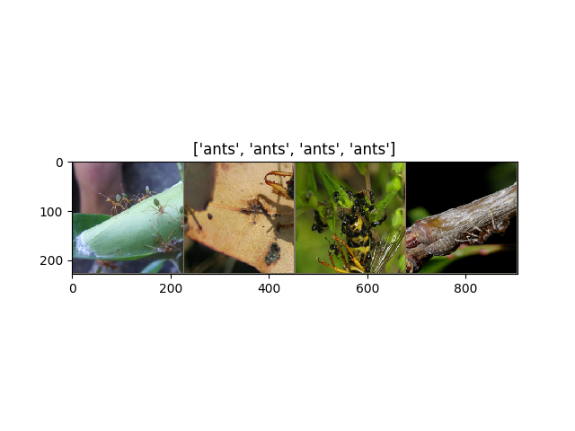
Visualize a few images

Let’s visualize a few training images so as to understand the data augmentations.

def imshow(inp, title=None):
    """Imshow for Tensor."""
    inp = inp.numpy().transpose((1, 2, 0))
    mean = np.array([0.485, 0.456, 0.406])
    std = np.array([0.229, 0.224, 0.225])
    inp = std * inp + mean
    inp = np.clip(inp, 0, 1)
    plt.imshow(inp)
    if title is not None:
        plt.title(title)
    plt.pause(0.001)  # pause a bit so that plots are updated


# Get a batch of training data
inputs, classes = next(iter(dataloaders['train']))

# Make a grid from batch
out = torchvision.utils.make_grid(inputs)

imshow(out, title=[class_names[x] for x in classes])

Training the model

Now, let’s write a general function to train a model. Here, we will illustrate:

• Scheduling the learning rate
• Saving the best model

In the following, parameter scheduler is an LR scheduler object from torch.optim.lr_scheduler.

def train_model(model, criterion, optimizer, scheduler, num_epochs=25):
    since = time.time()

    best_model_wts = copy.deepcopy(model.state_dict())
    best_acc = 0.0

    for epoch in range(num_epochs):
        print('Epoch {}/{}'.format(epoch, num_epochs - 1))
        print('-' * 10)

        # Each epoch has a training and validation phase
        for phase in ['train', 'val']:
            if phase == 'train':
                scheduler.step()
                model.train()  # Set model to training mode
            else:
                model.eval()   # Set model to evaluate mode

            running_loss = 0.0
            running_corrects = 0

            # Iterate over data.
            for inputs, labels in dataloaders[phase]:
                inputs = inputs.to(device)
                labels = labels.to(device)

                # zero the parameter gradients
                optimizer.zero_grad()

                # forward
                # track history if only in train
                with torch.set_grad_enabled(phase == 'train'):
                    outputs = model(inputs)
                    _, preds = torch.max(outputs, 1)
                    loss = criterion(outputs, labels)

                    # backward + optimize only if in training phase
                    if phase == 'train':
                        loss.backward()
                        optimizer.step()

                # statistics
                running_loss += loss.item() * inputs.size(0)
                running_corrects += torch.sum(preds == labels.data)

            epoch_loss = running_loss / dataset_sizes[phase]
            epoch_acc = running_corrects.double() / dataset_sizes[phase]

            print('{} Loss: {:.4f} Acc: {:.4f}'.format(
                phase, epoch_loss, epoch_acc))

            # deep copy the model
            if phase == 'val' and epoch_acc > best_acc:
                best_acc = epoch_acc
                best_model_wts = copy.deepcopy(model.state_dict())

        print()

    time_elapsed = time.time() - since
    print('Training complete in {:.0f}m {:.0f}s'.format(
        time_elapsed // 60, time_elapsed % 60))
    print('Best val Acc: {:4f}'.format(best_acc))

    # load best model weights
    model.load_state_dict(best_model_wts)
    return model

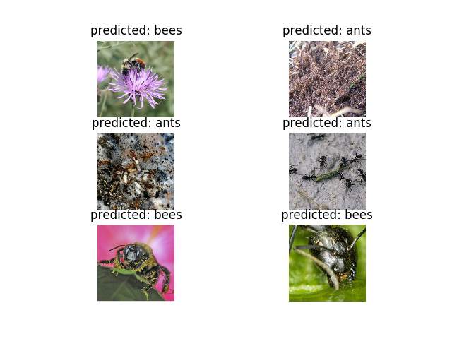
Visualizing the model predictions

Generic function to display predictions for a few images

def visualize_model(model, num_images=6):
    was_training = model.training
    model.eval()
    images_so_far = 0
    fig = plt.figure()

    with torch.no_grad():
        for i, (inputs, labels) in enumerate(dataloaders['val']):
            inputs = inputs.to(device)
            labels = labels.to(device)

            outputs = model(inputs)
            _, preds = torch.max(outputs, 1)

            for j in range(inputs.size()[0]):
                images_so_far += 1
                ax = plt.subplot(num_images//2, 2, images_so_far)
                ax.axis('off')
                ax.set_title('predicted: {}'.format(class_names[preds[j]]))
                imshow(inputs.cpu().data[j])

                if images_so_far == num_images:
                    model.train(mode=was_training)
                    return
        model.train(mode=was_training)

Finetuning the convnet

Load a pretrained model and reset final fully connected layer.

model_ft = models.resnet18(pretrained=True)
num_ftrs = model_ft.fc.in_features
model_ft.fc = nn.Linear(num_ftrs, 2)

model_ft = model_ft.to(device)

criterion = nn.CrossEntropyLoss()

# Observe that all parameters are being optimized
optimizer_ft = optim.SGD(model_ft.parameters(), lr=0.001, momentum=0.9)

# Decay LR by a factor of 0.1 every 7 epochs
exp_lr_scheduler = lr_scheduler.StepLR(optimizer_ft, step_size=7, gamma=0.1)

Train and evaluate

It should take around 15-25 min on CPU. On GPU though, it takes less than a minute.

model_ft = train_model(model_ft, criterion, optimizer_ft, exp_lr_scheduler,
                       num_epochs=25)

Out:

Epoch 0/24
----------
train Loss: 0.5540 Acc: 0.7336
val Loss: 0.2588 Acc: 0.8954

Epoch 1/24
----------
train Loss: 0.5288 Acc: 0.7910
val Loss: 0.3113 Acc: 0.9020

Epoch 2/24
----------
train Loss: 0.5715 Acc: 0.8074
val Loss: 0.2625 Acc: 0.8954

Epoch 3/24
----------
train Loss: 0.4685 Acc: 0.8361
val Loss: 0.5189 Acc: 0.8105

Epoch 4/24
----------
train Loss: 0.4609 Acc: 0.7951
val Loss: 0.3270 Acc: 0.8693

Epoch 5/24
----------
train Loss: 0.4258 Acc: 0.8402
val Loss: 0.2755 Acc: 0.8627

Epoch 6/24
----------
train Loss: 0.4301 Acc: 0.8320
val Loss: 0.2516 Acc: 0.9150

Epoch 7/24
----------
train Loss: 0.2645 Acc: 0.8975
val Loss: 0.2003 Acc: 0.9216

Epoch 8/24
----------
train Loss: 0.4231 Acc: 0.8197
val Loss: 0.1995 Acc: 0.9216

Epoch 9/24
----------
train Loss: 0.4237 Acc: 0.8484
val Loss: 0.2001 Acc: 0.9150

Epoch 10/24
----------
train Loss: 0.2910 Acc: 0.8607
val Loss: 0.1986 Acc: 0.9150

Epoch 11/24
----------
train Loss: 0.3015 Acc: 0.8852
val Loss: 0.1777 Acc: 0.9216

Epoch 12/24
----------
train Loss: 0.2800 Acc: 0.8934
val Loss: 0.1939 Acc: 0.9216

Epoch 13/24
----------
train Loss: 0.3545 Acc: 0.8320
val Loss: 0.2028 Acc: 0.9150

Epoch 14/24
----------
train Loss: 0.2652 Acc: 0.8893
val Loss: 0.1801 Acc: 0.9216

Epoch 15/24
----------
train Loss: 0.1955 Acc: 0.9221
val Loss: 0.1856 Acc: 0.9216

Epoch 16/24
----------
train Loss: 0.3078 Acc: 0.8402
val Loss: 0.2034 Acc: 0.9216

Epoch 17/24
----------
train Loss: 0.2575 Acc: 0.8893
val Loss: 0.1991 Acc: 0.9150

Epoch 18/24
----------
train Loss: 0.2993 Acc: 0.8730
val Loss: 0.1834 Acc: 0.9216

Epoch 19/24
----------
train Loss: 0.2655 Acc: 0.8852
val Loss: 0.1861 Acc: 0.9150

Epoch 20/24
----------
train Loss: 0.2295 Acc: 0.9098
val Loss: 0.2009 Acc: 0.9085

Epoch 21/24
----------
train Loss: 0.2719 Acc: 0.8811
val Loss: 0.1781 Acc: 0.9150

Epoch 22/24
----------
train Loss: 0.2683 Acc: 0.9057
val Loss: 0.1872 Acc: 0.9216

Epoch 23/24
----------
train Loss: 0.1990 Acc: 0.9262
val Loss: 0.2038 Acc: 0.9150

Epoch 24/24
----------
train Loss: 0.3078 Acc: 0.8443
val Loss: 0.1842 Acc: 0.9281

Training complete in 1m 15s
Best val Acc: 0.928105

visualize_model(model_ft)

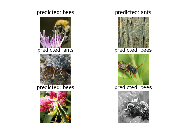
ConvNet as fixed feature extractor

Here, we need to freeze all the network except the final layer. We need to set requires_grad == False to freeze the parameters so that the gradients are not computed in backward().

You can read more about this in the documentation here.

model_conv = torchvision.models.resnet18(pretrained=True)
for param in model_conv.parameters():
    param.requires_grad = False

# Parameters of newly constructed modules have requires_grad=True by default
num_ftrs = model_conv.fc.in_features
model_conv.fc = nn.Linear(num_ftrs, 2)

model_conv = model_conv.to(device)

criterion = nn.CrossEntropyLoss()

# Observe that only parameters of final layer are being optimized as
# opoosed to before.
optimizer_conv = optim.SGD(model_conv.fc.parameters(), lr=0.001, momentum=0.9)

# Decay LR by a factor of 0.1 every 7 epochs
exp_lr_scheduler = lr_scheduler.StepLR(optimizer_conv, step_size=7, gamma=0.1)

Train and evaluate

On CPU this will take about half the time compared to previous scenario. This is expected as gradients don’t need to be computed for most of the network. However, forward does need to be computed.

model_conv = train_model(model_conv, criterion, optimizer_conv,
                         exp_lr_scheduler, num_epochs=25)

Out:

Epoch 0/24
----------
train Loss: 0.5684 Acc: 0.7008
val Loss: 0.2154 Acc: 0.9216

Epoch 1/24
----------
train Loss: 0.6135 Acc: 0.7213
val Loss: 0.2339 Acc: 0.9150

Epoch 2/24
----------
train Loss: 0.5376 Acc: 0.7746
val Loss: 0.1760 Acc: 0.9281

Epoch 3/24
----------
train Loss: 0.5482 Acc: 0.7746
val Loss: 0.4500 Acc: 0.8301

Epoch 4/24
----------
train Loss: 0.6307 Acc: 0.7336
val Loss: 0.1816 Acc: 0.9542

Epoch 5/24
----------
train Loss: 0.5348 Acc: 0.7541
val Loss: 0.2523 Acc: 0.9216

Epoch 6/24
----------
train Loss: 0.3509 Acc: 0.8566
val Loss: 0.2389 Acc: 0.9281

Epoch 7/24
----------
train Loss: 0.4197 Acc: 0.8320
val Loss: 0.1908 Acc: 0.9477

Epoch 8/24
----------
train Loss: 0.4030 Acc: 0.8156
val Loss: 0.1792 Acc: 0.9477

Epoch 9/24
----------
train Loss: 0.3229 Acc: 0.8484
val Loss: 0.1783 Acc: 0.9477

Epoch 10/24
----------
train Loss: 0.3085 Acc: 0.8648
val Loss: 0.1814 Acc: 0.9477

Epoch 11/24
----------
train Loss: 0.3339 Acc: 0.8402
val Loss: 0.1918 Acc: 0.9477

Epoch 12/24
----------
train Loss: 0.3329 Acc: 0.8402
val Loss: 0.1790 Acc: 0.9412

Epoch 13/24
----------
train Loss: 0.3591 Acc: 0.8320
val Loss: 0.1726 Acc: 0.9412

Epoch 14/24
----------
train Loss: 0.2591 Acc: 0.8975
val Loss: 0.1900 Acc: 0.9477

Epoch 15/24
----------
train Loss: 0.3220 Acc: 0.8484
val Loss: 0.1870 Acc: 0.9477

Epoch 16/24
----------
train Loss: 0.4379 Acc: 0.7910
val Loss: 0.1763 Acc: 0.9477

Epoch 17/24
----------
train Loss: 0.3358 Acc: 0.8402
val Loss: 0.2181 Acc: 0.9477

Epoch 18/24
----------
train Loss: 0.3809 Acc: 0.8279
val Loss: 0.2109 Acc: 0.9542

Epoch 19/24
----------
train Loss: 0.3471 Acc: 0.8484
val Loss: 0.1883 Acc: 0.9477

Epoch 20/24
----------
train Loss: 0.3506 Acc: 0.8525
val Loss: 0.1922 Acc: 0.9477

Epoch 21/24
----------
train Loss: 0.2658 Acc: 0.8975
val Loss: 0.1818 Acc: 0.9412

Epoch 22/24
----------
train Loss: 0.3664 Acc: 0.8279
val Loss: 0.1808 Acc: 0.9477

Epoch 23/24
----------
train Loss: 0.3049 Acc: 0.8852
val Loss: 0.2089 Acc: 0.9477

Epoch 24/24
----------
train Loss: 0.2753 Acc: 0.8811
val Loss: 0.1806 Acc: 0.9477

Training complete in 0m 38s
Best val Acc: 0.954248

visualize_model(model_conv)

plt.ioff()
plt.show()

Total running time of the script: ( 1 minutes 58.669 seconds)